Add total variance decomposition and computation of the coefficient of determination (make sure all your computations are done with online algorithms (e.g. with online algorithms (e.g. https://www.johndcook.com/blog/running_regression// etc.).
 'calcolo per il coefficiente di determinazione

        'Devianza totale
        Dim sum_ess As Double = 0
        For i_ess As Integer = 0 To y_est.Count - 1
            sum_ess += (y_est(i_ess) - current_onlineMeanY) * (y_est(i_ess) - current_onlineMeanY)
        Next

        'Devianza tra gruppi
        Dim sum_tss As Double = 0
        Dim y_obs As New List(Of Double)
        y_obs = listOfBDataP.Select(Function(p) p.x2).ToList
        For i_tss As Integer = 0 To y_obs.Count - 1
            sum_tss += (y_obs(i_tss) - current_onlineMeanY) * (y_obs(i_tss) - current_onlineMeanY)
        Next

        'Devianza entro i gruppi
        Dim sum_rss As Double = 0
        For i_rss As Integer = 0 To y_obs.Count - 1
            sum_rss += (y_obs(i_rss) - y_est(i_rss)) * (y_obs(i_rss) - y_est(i_rss))
        Next

        Dim coeffDet As Double = sum_ess / sum_tss
        Dim coeffDet2 As Double = 1 - sum_rss / sum_tss
Variance and covariance calculation (online algorithm)
 ...
        For Each d In listOfBDataP
            Calc_onlCov(d.x1, d.x2)
            Calc_onVar(d.x1)
        Next
...


 Public Sub Calc_onlCov(x As Double, y As Double)
        n += 1
        Dim dx As Double = x - meanX
        meanX += dx / CDbl(n)
        meanY += (y - meanY) / CDbl(n)
        b_online += dx * (y - meanY)
    End Sub

    Public Sub Calc_onVar(x As Double)
        n_v += 1
        Dim delta As Double = meanX_v + (x - meanX_v) / CDbl(n_v)
        sigma_online += (x - meanX_v) * (x - delta)
        meanX_v = delta
    End Sub
Generate and represent m paths of n point each (m, n are program parameters), where each point represents a pair of:
time index
relative frequency of success (i, f(i)) where f(i) is the sum of i Bernoulli random variables p^x(1-p)^(1-x) observed at the times j=1, …, i.
At time n (last time) and any other inner time 1<j<n (j is a program parameter) create and represent with histogram the distribution of f(i). At the same times (j and n), compute the absolute and relative frequency of the f(i)’s contained in the interval (p-ε, p+ε), where ε is a program parameter.
Do a research about the various methods proposed to compute the running median (one pass, online algorithms). Store (cite sources) the algorithm that you think is a good candidate and explaining briefly how it works and possibly show a quick demo.
The running median
The median of a set of integers is the midpoint value of the data set for which an equal number of integers are less than and greater than the value.
If we keep each number in a sorted sequence then cost of single entry is O(n) and finding median is O(n). A slight modification can be done by keeping the middle pointer and adjusting it based on the insertion on its left side and right side. In that case finding median after insertion is O(1). But the overall cost for finding median still remains O(n) as insertion in sorted sequence is necessary after each number is entered.
We can keep two heaps which divides the entered number in two almost equal halves. Half of the number would be greater than the median and the rest would be lesser. The upper half will be maintained in a min heap and the lower half will be maintained in a max heap. In this arrangement we can find out in O(1) time whether a new number would go to the upper half or lower half. All we need to do is to compare the new number with the head of two heaps. After deciding we can insert in a heap in O(log n) time. After this insertion if the heaps are unbalanced, we can just move from one heap to another. which is again of O(log n) complexity. And now we can find the median in O(1) time. If two heaps contain same number of elements then median is the average of the head of two heaps. If one is greater, then median is the head of the larger heap.
import java.util.Comparator;
import java.util.PriorityQueue;
import java.util.Random;


public class RunningMedian
{
    PriorityQueue<Integer> upperQueue;
    PriorityQueue<Integer> lowerQueue;

    public RunningMedian()
    {
        lowerQueue=new PriorityQueue<Integer>(
          20,new Comparator<Integer>()
        {

            @Override
            public int compare(Integer o1, Integer o2)
            {

                return -o1.compareTo(o2);
            }

        });
        upperQueue=new PriorityQueue<Integer>();
        upperQueue.add(Integer.MAX_VALUE);
        lowerQueue.add(Integer.MIN_VALUE);
    }

    public double getMedian(int num)
    {
        //adding the number to proper heap
            if(num>=upperQueue.peek())
                upperQueue.add(num);
            else
                lowerQueue.add(num);
        //balancing the heaps
        if(upperQueue.size()-lowerQueue.size()==2)
            lowerQueue.add(upperQueue.poll());
        else if(lowerQueue.size()-upperQueue.size()==2)
            upperQueue.add(lowerQueue.poll());
        //returning the median
        if(upperQueue.size()==lowerQueue.size())
            return(upperQueue.peek()+lowerQueue.peek())/2.0;
        else if(upperQueue.size()>lowerQueue.size())
            return upperQueue.peek();
        else
            return lowerQueue.peek();

    }
    public static void main(String[] args)
    {
        Random random=new Random();
        RunningMedian runningMedian=new RunningMedian();
        System.out.println("num\tmedian");
        for(int i=0;i<50;++i)
        {
            int num=random.nextInt(100);
            System.out.print(num);
            System.out.print("\t");
            System.out.println(
              runningMedian.getMedian(num));
        }

    }

}
1) illustrates with visual evidence the law of large numbers LLN, and the various definitions of convergence 2) illustrates the binomial distribution 3) illustrates the convergence of the binomial to the normal 4) illustrates the central limit theorem 5) provides a basic example of stochastic process (sequence of r.v.’s defined on the same probability space)
LLN–Law of large numbers
Is a theorem that describes the result of performing the same experiment a large number of times. According to the law, the average of the results obtained from a large number of trials should be close to the expected value and will tend to become closer to the expected value as more trials are performed.
The expected value of a random variable , denoted ,is a generalization of the weighted average and is intuitively the arithmetic mean of a large number of independentrealizations of .
the expected value of a constant random variable is
the expected value of a random variable with equiprobable outcomes is defined as the arithmetic mean of the terms
If some of the probabilities of an individual outcome are unequal, then the expected value is defined to be the probability-weighted average of the , that is, the sum of the products . The expected value of a general random variable involves integration in the sense of Lebesgue.
The LLN is important because it guarantees stable long-term results for the averages of some random events.
While a casino may lose money in a single spin of the roulette wheel, its earnings will tend towards a predictable percentage over a large number of spins. Any winning streak by a player will eventually be overcome by the parameters of the game.
It is important to remember that the law only applies (as the name indicates) when a large number of observations is considered. There is no principle that a small number of observations will coincide with the expected value or that a streak of one value will immediately be “balanced” by the others. (The gambler’s fallacy, also known as the Monte Carlo fallacy, is the erroneous belief that if a particular event occurs more frequently than normal during the past it is less likely to happen in the future (or vice versa), when it has otherwise been established that the probability of such events does not depend on what has happened in the past.)
In the repeated toss of a fair coin, the outcomes in different tosses are statistically independent and the probability of getting heads on a single toss is 1/2. Since the probability of a run of five successive heads is 1/32, a person might believe that the next flip would be more likely to come up tails rather than heads again. This is incorrect and is an example of the gambler’s fallacy. The event “5 heads in a row” and the event “first 4 heads, then a tails” are equally likely, each having probability 1/32. Since the first four tosses turn up heads, the probability that the next toss is a head is: .
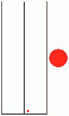
Simulation of coin tosses: Each frame, a coin is flipped which is red on one side and blue on the other. The result of each flip is added as a coloured dot in the corresponding column. As the pie chart shows, the proportion of red versus blue approaches 50-50 (the law of large numbers). But the difference between red and blue does not systematically decrease to zero.
Convergence concepts in probability
Converge in distribution
The r.v.s Xn converge in distribution to r.v. X if
Converge in distribution
Converge in probability
The r.v.s Xn converge in probability to r.v. X if for all ε > 0
Converge in probability
Converges almost surely
The r.v.s Xn converge in almost surely to r.v. X if
Converge almost surely
If Xn converges almost surely to X, then it also converges in probability. If Xn converges in probability to X, then it also converges in distribution.
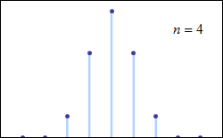
The binomial distribution
A binomial distribution is a type of distribution that has two possible outcomes. Let p be the probability of success and q (=1−p) be the probability of failure. The binomial distribution is the probability distribution of the number x of successful trials in n Bernoulli trials and is denoted by Bi(n,p).
The binomial distribution is closely related to the Bernoulli distribution, the Bernoulli distribution is the Binomial distribution with n=1.
For example, a coin toss has only two possible outcomes: heads or tails and taking a test could have two possible outcomes: pass or fail.
The probability of having x successful trials is given by px, while the probability of having n−x unsuccessful trials is given by q(n−x). The number of combinations of x successful trials and n−x unsuccessful trials is given by
The binomial coefficient
The binomial distribution formula can calculate the probability of success for binomial distributions
Binomial distributions must also meet the following three criteria:
It starts at 0 because the first flip happened to be tails
The number of observations or trials is fixed. In other words, you can only figure out the probability of something happening if you do it a certain number of times. This is common sense—if you toss a coin once, your probability of getting a heads is 50%. If you toss a coin a 20 times, your probability of getting a heads is very, very close to 100%.
Each observation or trial is independent. In other words, none of your trials have an effect on the probability of the next trial.
The probability of success (tails, heads, fail or pass) is exactly the same from one trial to another.
The central limit theorem
The central limit theorem (CLT) establishes that, in many situations, when independent random variables are added, their properly normalized sum tends toward a normal distribution (informally a bell curve) even if the original variables themselves are not normally distributed.
A normaldistribution is a type of continuous probability distribution for a real-valued random variable.
If X1 , . . . , Xn are random samples each of size n taken from a population with overall mean μ and finite variance σ2 and if is the sample mean, the limiting form of the distribution of
as n → ∞ , is the standard normal distribution.
For example, suppose that a sample is obtained containing many observations, each observation being randomly generated in a way that does not depend on the values of the other observations, and that the arithmetic mean of the observed values is computed. If this procedure is performed many times, the central limit theorem says that the probability distribution of the average will closely approximate a normal distribution. A simple example of this is that if one flips a coin many times, the probability of getting a given number of heads will approach a normal distribution, with the mean equal to half the total number of flips. At the limit of an infinite number of flips, it will equal a normal distribution.
The central limit theorem has several variants: one of this, the de Moivre–Laplace theorem, says that normal distribution may be used as an approximation to the binomial distribution.
The de Moivre–Laplace theorem, which is a special case of the central limit theorem, states that the normal distribution may be used as an approximation to the binomial distribution under certain conditions.
Consider a series of n independent trials, each resulting in one of two possible outcomes, a success with probability p (0 < p < 1) and failure with probability q = 1-p. Let Xn denote the number of successes in these n trials. Then the random variable(r.v.) Xn is said to have binomial distribution with parameters n and p, b(n,p).
So
The probability density(or mass) function (pdf) of Xn is given by:
with sum(pn(x) = 1) for x = 0,…,n
The mean and variance of the binomial r.v. Xn are given, respectively, by:
E[Xn] = μ = np
Var[Xn] = σ² = npq = np(1-p)
For sufficiently large n, the following random variable has a standard normal distribution:
That is:
The general form of Normal distribution probability density function is:
Notation: N(μ,σ²)
For a binomial distribution, as n grows large, for k in the neighborhood of np we can approximate:
Pdf of binomial converge to a normal. N(0,1)
in the sense that the ratio of the left-hand side to the right-hand side converges to 1 as n → ∞.
(The normal distribution is generally considered to be a pretty good approximation for the binomial distribution when np ≥ 5 and n(1 – p) ≥ 5)
Stochastic process
Also called random process, is a mathematical object usually defined as a family of random variables. Many stochastic processes can be represented by time series. However, a stochastic process is by nature continuous while a time series is a set of observations indexed by integers. A stochastic process may involve several related random variables. The term random function is also used to refer to a stochastic or random process, because a stochastic process can also be interpreted as a random element in a function space.
One of the simplest stochastic processes is the Bernoulli process(discrete-time stochastic process), which is a sequence of independent and identically distributed (iid) random variables, where each random variable takes either the value one or zero, say one with probability p and zero with probability 1 − p.
This process can be linked to repeatedly flipping a coin, where the probability of obtaining a head is p and its value is one, while the value of a tail is zero.In other words, a Bernoulli process is a sequence of iid Bernoulli random variables, where each coin flip is an example of a Bernoulli trial.


 , denoted
 ![E[X]](https://wikimedia.org/api/rest_v1/media/math/render/svg/e455a34363c03fc5df8208d8b81fa29e3cdd524e) , is a generalization of the weighted average and is intuitively the arithmetic mean of a large number of independentrealizations of
, is a generalization of the weighted average and is intuitively the arithmetic mean of a large number of independentrealizations of  is
is 
 is defined as the arithmetic mean of the terms
 of an individual outcome
  are unequal, then the expected value is defined to be the probability-weighted average of the
  products
  . The expected value of a general random variable involves integration in the sense of Lebesgue.
 .
.


 is the sample mean, the limiting form of the distribution of