Homework15_R

Explain how parametric inference works and the main ideas of statistical induction, including the role of Bayes theorem and the different approach between “bayesian” and “frequentist”.

Inferential statistics

You have a population which is too large to study fully, so you use statistical techniques to estimate its properties from samples taken from that population.
So, in inferential statistics, we try to infer something about a population from data coming from a sample taken from it. We need the concept of probability.

Statistical inference is a particular frame of Statistical induction.
Induction is a method of reasoning in which the premises are viewed as supplying some evidence, but not full assurance, for the truth of the conclusion. Inductive reasoning is distinct from deductive reasoning, where the conclusion of a deductive argument is certain.

Parametric statistics is a branch of statistics which assumes that sample data comes from a population that can be adequately modeled by a probability distribution that has a fixed set of parameters.
Example:
The normal family of distributions all have the same general shape and are parameterized by mean and standard deviation. That means that if the mean and standard deviation are known and if the distribution is normal, the probability of any future observation lying in a given range is known.

Frequentist and bayesian approach

https://www.probabilisticworld.com/frequentist-bayesian-approaches-inferential-statistics/

The problem is that we don’t know the prior probability. So, the inferential statistics splits in two:

• give it an uniform distribution
• give it a shape

The frequentist way

Sampling is infinite and decision rules can be sharp. Data are a repeatable random sample – there is a frequency. Underlying parameters are fixed i.e. they remain constant during this repeatable sampling process.

The Bayesian way

Unknown quantities are treated probabilistically and the state of the world can always be updated. Data are observed from the realised sample. Parameters are unknown and described probabilistically. It is the data which are fixed.

Are you a Bayesian or a Frequentist?

You have a coin that when flipped ends up head with probability p and ends up tail with probability 1−p. (The value of p is unknown.)

Trying to estimate p, you flip the coin 14 times. It ends up head 10 times.

Then you have to decide on the following event: “In the next two tosses we will get two heads in a row.”

Would you bet that the event will happen or that it will not happen?

Using frequentist statistics, we would say that the best (maximum likelihood) estimate for p is p=10/14.
In this case, the probability of two heads is 0.714

The Bayesian approach, instead, treat p as a random variable with its own distribution of possible values.
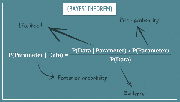
The distribution can be defined by the existing evidence. The logic goes as follows. What is the probability of a given value of p, given the data? We find it, with the Bayes thm.

https://www.behind-the-enemy-lines.com/2008/01/are-you-bayesian-or-frequentist-or.html

https://www.youtube.com/watch?v=TSkDZbGS94k
https://en.wikipedia.org/wiki/Confidence_interval
https://link.springer.com/chapter/10.1007/978-0-387-09612-4_9
https://en.wikipedia.org/wiki/Frequentist_inference
https://www.nasa.gov/consortium/FrequentistInference
https://en.wikipedia.org/wiki/Bayesian_inference
https://en.wikipedia.org/wiki/Parametric_statistics
https://en.wikipedia.org/wiki/Inductive_reasoning
https://stats.stackexchange.com/questions/22/bayesian-and-frequentist-reasoning-in-plain-english

Homework10_R

Explain a unified conceptual framework to obtain all most common measures of central tendency using the concept of distance (or “premetric” in general).

Measures of Central Tendency

A measure of central tendency is a single value that attempts to describe a set of data by identifying the central position within that set of data. As such, measures of central tendency are sometimes called measures of central location. They are also classed as summary statistics.

The p-norm and L^p spaces

(every vector from the origin to the unit circle has a length of one, the length being calculated with length-formula of the corresponding p).

For a real number p ≥ 1, the p-norm or L^p-norm of x is defined by:

The Euclidean norm from above falls into this class and is the 2-norm, and the 1-norm is the norm that corresponds to the rectilinear distance (Manhattan distance).

The length of a vector x = (x₁, x₂, …, x_n) in the n-dimensional real vector space Rⁿ is usually given by the Euclidean norm:

The Euclidean distance between two points x and y is the length ||x − y||₂ of the straight line between the two points.

The function: defines a metric.

The L^p spaces are function spaces defined using a natural generalization of the p-norm for finite-dimensional vector spaces.
In statistics, measures of central tendency and statistical dispersion, such as the mean, median, and standard deviation, are defined in terms of L^p metrics, and measures of central tendency can be characterized as solutions to variational problems, in the sense of the calculus of variations, namely minimizing variation from the center.
In the sense of L^p spaces, the correspondence is:

In equations, for a given (finite) data set X, thought of as a vector x = (x₁,…,x_n), the dispersion about a point c is the “distance” from x to the constant vector c = (c,…,c) in the p-norm (normalized by the number of points n):

For p = 0 and p = +-∞ these functions are defined by taking limits.

Clustering

Instead of a single central point, one can ask for multiple points such that the variation from these points is minimized. This leads to cluster analysis, where each point in the data set is clustered with the nearest “center”.

Mode, median and mean

Hence, measures of central tendency help you find the middle, or the average, of a data set. The 3 most common measures of central tendency are the

• mode: the most frequent value.
• median: the middle number in an ordered data set.
• mean: the sum of all values divided by the total number of value.

https://www.scribbr.com/statistics/central-tendency/
https://en.wikipedia.org/wiki/Lp_space#The_p-norm_in_finite_dimensions
https://en.wikipedia.org/wiki/Central_tendency

Homework11_R

What are the most common types of means known? Find one example where these two types of means arise naturally: geometric, harmonic.

General or power mean

In mathematics, generalized means (or power mean) are a family of functions for aggregating sets of numbers, that include as special cases the Pythagorean means (arithmetic, geometric, and harmonicmeans).
The generalized mean or power mean is:

Special cases:
https://en.wikipedia.org/wiki/Generalized_mean#Special_cases

Arithmetic mean

It is generally referred as the average or simply mean. (p = 1).

Geometric mean

It indicates the central tendency or typical value of a set of numbers by using the product of their values (When p -> 0):

The geometric mean can be understood in terms of geometry. The geometric mean of two numbers, and b , is the length of one side of a square whose area is equal to the area of a rectangle with sides of lengths and .
The geometric mean is used in finance to calculate average growth rates and is referred to as the compounded annual growth rate.

Harmonic Mean

Typically, it is appropriate for situations when the average of rates is desired(p = -1):

In computer science, specifically information retrieval and machine learning, the harmonic mean of the precision (true positives per predicted positive) and the recall (true positives per real positive) is often used as an aggregated performance score for the evaluation of algorithms and systems: the F-score (or F-measure). This is used in information retrieval because only the positive class is of relevance, while number of negatives, in general, is large and unknown.
The weighted harmonic mean is used in finance to average multiples like the price-earnings ratio because it gives equal weight to each data point.

https://en.wikipedia.org/wiki/Geometric_mean
https://www.investopedia.com/ask/answers/060115/what-are-some-examples-applications-geometric-mean.asp
https://econtutorials.com/blog/mean-and-its-types-in-statistics/
https://en.wikipedia.org/wiki/Harmonic_mean
https://www.investopedia.com/terms/h/harmonicaverage.asp

Homework12_R

Explain the idea underlying the measures of dispersion and the reasons of their importance.

Dispersion

In statistics, dispersion (also called variability, scatter, or spread) is the extent to which a distribution is stretched or squeezed or, also, is a way of describing how spread out a set of data is. Common examples of measures of statistical dispersion are the variance and standard deviation.

Example of samples from two populations with the same mean but different dispersion. The red population is much more dispersed than the yellow population.

Dispersion is contrasted with location or central tendency, and together they are the most used properties of distributions.

Some measures of the dispersion

Range: is the simple measure of dispersion, which is defined as the difference between the largest value and the smallest value.

Standard Deviation: the most used method, It is a measure of spread of data about the mean.

Why necessary?

While measures of central tendency are used to estimate “normal” values of a dataset, measures of dispersion are important for describing the spread of the data, or its variation around a central value.
Two distinct samples may have the same mean or median, but completely different levels of variability, or vice versa. A proper description of a set of data should include both of these characteristics.

When it comes to samples, that dispersion is important because it determines the margin of error you’ll have when making inferences about measures of central tendency, like averages.
Show you the variability of your data. 

https://en.wikipedia.org/wiki/Statistical_dispersion
https://iridl.ldeo.columbia.edu/dochelp/StatTutorial/Dispersion/index.html
https://www.statisticssolutions.com/dispersion/
https://exploringyourmind.com/measures-of-dispersion-in-statistics/

Homework13_R

Find out all the most important properties of the linear regression.

What is it?

In statistics, is a linear approach to modeling the relationship between a scalar response (or dependent variable) and one or more explanatory variables (or independent variables).

Linear regression finds the straight line, LSRL, that best represents observations in a bivariate data set.
Suppose Y is a dependent variable, and X is an independent variable. The population regression line is:

Y = a + bX

where ‘a‘ is a constant and ‘b‘ the regression coefficient(in relationship to the angular coefficient).

The regression line has the following properties:

• The line minimizes the sum of squared differences between observed values and predicted values
• The regression line passes through the mean of the X values and through the mean of the Y values
• The regression constant (a) is equal to the y intercept of the regression line.
• The regression coefficient (b) is the average change in the dependent variable (Y) for a 1-unit change in the independent variable (X). It is the slope of the regression line.

https://en.wikipedia.org/wiki/Linear_regression
https://www.tandfonline.com/doi/abs/10.1080/00220671.1947.10881608?journalCode=vjer20
https://stattrek.com/regression/linear-regression.aspx

Homework9_R

Do a review about charts useful for statistics and data presentation (example of some: StatCharts.txt ). What is the chart type that impressed you most and why ?

What is Data Visualization?

The human mind is very receptive to visual information. That’s why data visualization is a powerful tool for communication.    

Data visualization is the visual presentation of data or information. The goal of data visualization is to communicate data or information clearly and effectively to readers. Typically, data is visualized in the form of a chart, infographic, diagram or map. 

Charts use visual symbols like line, bars, dots, slices, and icons to represent data points. 

What type of chart should I use to visualize my data? Does it matter?

Yes, it matters. Choosing a type of chart that doesn’t work with your data can end up misrepresenting and skewing your data. 

Pie charts display portions of a whole. A pie chart works when you want to compare proportions that are substantially different. But when your proportions are similar, a pie chart can make it difficult to tell which slice is bigger than the other. That’s why, in most other cases, a bar chart is a safer bet.

I have often used pie charts or column charts. But in a university course I had the need to use the bubble chart, programming the filling of the ‘buckets’ myself in matlab, thus being able to have information clearly, through the size of these bubbles. Very cool!

https://venngage.com/blog/data-visualization/

Homework8_R

Explain the concept of statistical independence and why, in case of independence, the relative joint frequencies are equal to the products of the corresponding marginal frequencies.

Statistical independence and marginal frequencies

If the frequency, for alla i, of xi fixed yj is equal for all j and is also equal to the marginal, then x and y are indipendent.

This can be seen more easily by looking the shape, that are the same, for all fixed Y or X.
It is therefore obvious that one variable does not depend on the other.

F(x,y) is the joint distribution function and Fx and Fy are the marginal ones.

https://math.stackexchange.com/questions/1789265/understanding-statistical-independence-of-events-using-a-relative-frequency-inte

https://www.researchgate.net/post/Why_is_it_so_that_only_for_bivariate_multivariate_normal_uncorrelated_distribution_implies_independence_and_not_other_distribution

Homework7_R

Explain what are marginal, joint and conditional distributions and how we can explain the Bayes theorem using relative frequencies.

Why different distributions

When we have a bivariate distribution, we can represent it with a Contingency table. In this table we can define different type of distribution.

Marginal Distribution

The marginal distribution take us back to the univariate case (we ignore the other variable) and is called marginal because in the contingency table is a the marginal.

Specifically, the relative marginal frequencies of X are defined as:

and of Y:

Join Distribution

The join distribution is the element nij in the table. And it represent how many times a combination of two conditions happens together.

Conditional Distribution

The conditional frequency distribution of Y given X is the frequency distribution of Y when X is known to be a particular value.

The conditional frequency distribution of X given Y is the frequency distribution of X when Y is known to be a particular value.

The distribution is constrained by the fact that they fall into the fixed class (of x or y)

Relative Frequency

With this definition we can say:

The Bayes Thm

http://www.est.uc3m.es/esp/nueva_docencia/comp_col_get/lade/estadistica_I/doc_generica/Tema3inglesImp.pdf
https://en.wikipedia.org/wiki/Bayes%27_theorem

Homework6_R

Show how we can obtain an online algo for the arithmetic mean and explain the various possible reasons why it is preferable to the “naive” algo based on the definition.

Online Algorithm

An online problem is a problem where the size of the input is not known in advance. An algorithm that solves an online problem by continous calculation (after each single input) is called an online algorithm.

Algorithm for Arithmetic mean

The usual way to calculate the average for a set of data is:

This naive approach to obtain the mean have a couple of limitations in practice:

• We accumulate a potentially large sum, whic can cause precision and overflows problems when using floating point types.
• We need to have all of the data available before we can do the calculation!

Both of these problems can be solved with an incremental approach where we adjust the average for each new value that comes along:

Let’s start with the formula for the average that we saw earlier:

Let’s split up the sum so that we add up the first n-1 values first, and then we add the last value x_n.

We know that the average = total / count:

Let’s rearrange this a bit:

Here’s the result of applying the above substitution to the total of the first n-1 values:

Let’s expand this:

Rearranging a bit, we get:

We can cancel out the n’s in the first fraction to obtain our final result:

So, the strategy for an online algorithm is to hold some current value for the average(i.e the precedent mean).

Observing the naive method, we see easily that if some values ​​are too large or if we add infinite ones we will arrive at the overflow or we will have problems with bad approximation, instead with the second method (studied by Knuth) we always add a small contribution, because the added contribution is the difference between the last observation and the first one, divided by N. The larger N is, the smaller it will be.

https://nestedsoftware.com/2018/03/20/calculating-a-moving-average-on-streaming-data-5a7k.22879.html
https://en.wikipedia.org/wiki/Kahan_summation_algorithm

Homework5_R

Describe the most common configuration of data repository in the real world and corporate environment. Concepts such as Operation systems (oltp), Data Warehouse DW, Data Marts, Analitical and statistical systems (olap), etc. Try to draw a conceptual picture of how all these elements works toghether and how the flow of data and informations is processed to extract useful knowledge from raw data.

It’s one thing to collect and store data
it’s another to accurately decipher what the data is saying

“Statistics are like bikinis. What they reveal is suggestive, but what they conceal is vital.”
Aaron Levenstein, Business Professor at Baruch College

Successful organizations continue to derive business value from their data. One of the first steps towards a successful big data strategy is choosing the underlying technology of how data will be stored, searched, analyzed, and reported on.

Data repository

A data repository is also known as a data library or data archive. Is a large database infrastructure that collect, manage, and store data sets for data analysis, sharing and reporting.
Examples are:

• data warehouse
• data lake
• data marts

We have a source of data (i.e. Businesses), that with a stream store the data in a repository (i.e. Data Lake).

OLTP(On-line Transaction Processing) is the operation systems that provide source data to data repository such as Data Lake.

Data lakes are a great way to store huge amounts of data and drive business insights. But they have limited governance and weak traceability, lineage, and quality. Many lakes have turned into swamps, that is a storage more confusionary.

With some operations, i.e. ETL(Extraxt, Trasform and Load) or ELT, we can build and store the data in Data Warehouse, a more organized data repository.

Data Warehouse stores data in files or folders which helps to organize and use the data to take strategic decisions.

From Data Warehouse we can create another kind of repository that are most focus on specific task: Data Marts.

From Data Marts we have operation systems that analize the data, i.e. OLAP (On-line Analytical Processing)

Conclusions

Data lakes offer the flexibility of storing raw data, including all the meta data and a schema can be applied when extracting the data to be analyzed. Databases and Data Warehouses require ETL processes where the raw data is transformed into a pre-determined structure, also known as, schema-on-write.
Data warehouses typically deal with large data sets, but data analysis requires easy-to-find and readily available data. That’s why smart companies use data marts.
The data marts are one key to efficiently transforming information into insights.

Even with the improved flexibility and efficiency that data marts offer, big data—and big business—is still becoming too big for many on-premises solutions. As data warehouses and data lakes move to the cloud, so too do data marts.

Sources:

Data Repository

OLTP and OLAP

ELT and ETL

https://www.mackenziecorp.com/much-data-not-enough-data-lets-start/
https://www.confluent.io/learn/database-data-lake-data-warehouse-compared/
https://www.talend.com/resources/what-is-data-mart/