Dim x_prec As Double = listOfBDataP(0).x1
        Dim y_dipPrec As Double = a + b * x_prec

        For Each d In listOfBDataP.Skip(1)
            Dim y_dipCurr As Double = a + b * d.x1
            Dim p_xPrec As Double = X_Viewport(x_prec, viewport, min_x, range_x)
            Dim p_yPrec As Double = Y_Viewport(y_dipPrec, viewport, min_y, range_y)
            Dim p_xCurr As Double = X_Viewport(d.x1, viewport, min_x, range_x)
            Dim p_yCurr As Double = Y_Viewport(y_dipCurr, viewport, min_y, range_y)
            gc.DrawLine(Pens.Red, New Point(p_xPrec, p_yPrec), New Point(p_xCurr, p_yCurr))
            x_prec = d.x1
            y_dipPrec = y_dipCurr
        Next
where
b = COV(X,Y)/variance a = y – bx (y and x are the average of Y and X value)
Remember:
Variance
Covariance
  Dim sigma = calc_var()
        Dim b As Double = Calc_cov() / sigma
        Dim a As Double = current_onlineMeanY - b * current_onlineMeanX
  Public Function Calc_cov() As Double
        Dim sum As Double
        Dim n As Double = listOfBDataP.Count
        For Each d In listOfBDataP
            sum += d.x1 * d.x2
        Next
        Return (sum - n * current_onlineMeanX * current_onlineMeanY) / (n - 1)
    End Function

    Public Function Calc_var() As Double
        Dim sigma As Double
        For Each d In listOfBDataP
            sigma += Math.Pow((d.x1 - current_onlineMeanX), 2)
        Next

        Return sigma / (listOfBDataP.Count - 1)
    End Function
1) illustrates with visual evidence the law of large numbers LLN, and the various definitions of convergence 2) illustrates the binomial distribution 3) illustrates the convergence of the binomial to the normal 4) illustrates the central limit theorem 5) provides a basic example of stochastic process (sequence of r.v.’s defined on the same probability space)
LLN–Law of large numbers
Is a theorem that describes the result of performing the same experiment a large number of times. According to the law, the average of the results obtained from a large number of trials should be close to the expected value and will tend to become closer to the expected value as more trials are performed.
The expected value of a random variable , denoted ,is a generalization of the weighted average and is intuitively the arithmetic mean of a large number of independentrealizations of .
the expected value of a constant random variable is
the expected value of a random variable with equiprobable outcomes is defined as the arithmetic mean of the terms
If some of the probabilities of an individual outcome are unequal, then the expected value is defined to be the probability-weighted average of the , that is, the sum of the products . The expected value of a general random variable involves integration in the sense of Lebesgue.
The LLN is important because it guarantees stable long-term results for the averages of some random events.
While a casino may lose money in a single spin of the roulette wheel, its earnings will tend towards a predictable percentage over a large number of spins. Any winning streak by a player will eventually be overcome by the parameters of the game.
It is important to remember that the law only applies (as the name indicates) when a large number of observations is considered. There is no principle that a small number of observations will coincide with the expected value or that a streak of one value will immediately be “balanced” by the others. (The gambler’s fallacy, also known as the Monte Carlo fallacy, is the erroneous belief that if a particular event occurs more frequently than normal during the past it is less likely to happen in the future (or vice versa), when it has otherwise been established that the probability of such events does not depend on what has happened in the past.)
In the repeated toss of a fair coin, the outcomes in different tosses are statistically independent and the probability of getting heads on a single toss is 1/2. Since the probability of a run of five successive heads is 1/32, a person might believe that the next flip would be more likely to come up tails rather than heads again. This is incorrect and is an example of the gambler’s fallacy. The event “5 heads in a row” and the event “first 4 heads, then a tails” are equally likely, each having probability 1/32. Since the first four tosses turn up heads, the probability that the next toss is a head is: .
Simulation of coin tosses: Each frame, a coin is flipped which is red on one side and blue on the other. The result of each flip is added as a coloured dot in the corresponding column. As the pie chart shows, the proportion of red versus blue approaches 50-50 (the law of large numbers). But the difference between red and blue does not systematically decrease to zero.
Convergence concepts in probability
Converge in distribution
The r.v.s Xn converge in distribution to r.v. X if
Converge in distribution
Converge in probability
The r.v.s Xn converge in probability to r.v. X if for all ε > 0
Converge in probability
Converges almost surely
The r.v.s Xn converge in almost surely to r.v. X if
Converge almost surely
If Xn converges almost surely to X, then it also converges in probability. If Xn converges in probability to X, then it also converges in distribution.
The binomial distribution
A binomial distribution is a type of distribution that has two possible outcomes. Let p be the probability of success and q (=1−p) be the probability of failure. The binomial distribution is the probability distribution of the number x of successful trials in n Bernoulli trials and is denoted by Bi(n,p).
The binomial distribution is closely related to the Bernoulli distribution, the Bernoulli distribution is the Binomial distribution with n=1.
For example, a coin toss has only two possible outcomes: heads or tails and taking a test could have two possible outcomes: pass or fail.
The probability of having x successful trials is given by px, while the probability of having n−x unsuccessful trials is given by q(n−x). The number of combinations of x successful trials and n−x unsuccessful trials is given by
The binomial coefficient
The binomial distribution formula can calculate the probability of success for binomial distributions
Binomial distributions must also meet the following three criteria:
It starts at 0 because the first flip happened to be tails
The number of observations or trials is fixed. In other words, you can only figure out the probability of something happening if you do it a certain number of times. This is common sense—if you toss a coin once, your probability of getting a heads is 50%. If you toss a coin a 20 times, your probability of getting a heads is very, very close to 100%.
Each observation or trial is independent. In other words, none of your trials have an effect on the probability of the next trial.
The probability of success (tails, heads, fail or pass) is exactly the same from one trial to another.
The central limit theorem
The central limit theorem (CLT) establishes that, in many situations, when independent random variables are added, their properly normalized sum tends toward a normal distribution (informally a bell curve) even if the original variables themselves are not normally distributed.
A normaldistribution is a type of continuous probability distribution for a real-valued random variable.
If X1 , . . . , Xn are random samples each of size n taken from a population with overall mean μ and finite variance σ2 and if is the sample mean, the limiting form of the distribution of
as n → ∞ , is the standard normal distribution.
For example, suppose that a sample is obtained containing many observations, each observation being randomly generated in a way that does not depend on the values of the other observations, and that the arithmetic mean of the observed values is computed. If this procedure is performed many times, the central limit theorem says that the probability distribution of the average will closely approximate a normal distribution. A simple example of this is that if one flips a coin many times, the probability of getting a given number of heads will approach a normal distribution, with the mean equal to half the total number of flips. At the limit of an infinite number of flips, it will equal a normal distribution.
The central limit theorem has several variants: one of this, the de Moivre–Laplace theorem, says that normal distribution may be used as an approximation to the binomial distribution.
The de Moivre–Laplace theorem, which is a special case of the central limit theorem, states that the normal distribution may be used as an approximation to the binomial distribution under certain conditions.
Consider a series of n independent trials, each resulting in one of two possible outcomes, a success with probability p (0 < p < 1) and failure with probability q = 1-p. Let Xn denote the number of successes in these n trials. Then the random variable(r.v.) Xn is said to have binomial distribution with parameters n and p, b(n,p).
So
The probability density(or mass) function (pdf) of Xn is given by:
with sum(pn(x) = 1) for x = 0,…,n
The mean and variance of the binomial r.v. Xn are given, respectively, by:
E[Xn] = μ = np
Var[Xn] = σ² = npq = np(1-p)
For sufficiently large n, the following random variable has a standard normal distribution:
That is:
The general form of Normal distribution probability density function is:
Notation: N(μ,σ²)
For a binomial distribution, as n grows large, for k in the neighborhood of np we can approximate:
Pdf of binomial converge to a normal. N(0,1)
in the sense that the ratio of the left-hand side to the right-hand side converges to 1 as n → ∞.
(The normal distribution is generally considered to be a pretty good approximation for the binomial distribution when np ≥ 5 and n(1 – p) ≥ 5)
Stochastic process
Also called random process, is a mathematical object usually defined as a family of random variables. Many stochastic processes can be represented by time series. However, a stochastic process is by nature continuous while a time series is a set of observations indexed by integers. A stochastic process may involve several related random variables. The term random function is also used to refer to a stochastic or random process, because a stochastic process can also be interpreted as a random element in a function space.
One of the simplest stochastic processes is the Bernoulli process(discrete-time stochastic process), which is a sequence of independent and identically distributed (iid) random variables, where each random variable takes either the value one or zero, say one with probability p and zero with probability 1 − p.
This process can be linked to repeatedly flipping a coin, where the probability of obtaining a head is p and its value is one, while the value of a tail is zero.In other words, a Bernoulli process is a sequence of iid Bernoulli random variables, where each coin flip is an example of a Bernoulli trial.
Make a short demonstrative program where you apply both the Riemann and Lebesgue approach to integration to compute numerically (with an increasingly large number of subdivisions) the integral on a bounded continuous function of your choice and compare the results. [Optionally, show with an animation, using the graphics object, the convergence to a limit, as the number of subdivisions of the function domain (for Riemann) or range (for Lebesgue) increases.]
Riemann integral(left) and Lesbesgue integral(right)
'take x_1 and x_2 that denote 'the range of function' in x axis
'take interval to divide the axis(in this case y axis)
'take function f to map the x in y axis with respect to the given function
'take g as inverse to f to return to the x axis

Public Function Lebesgue_int(x_1 As Integer, x_2 As Integer, interval As Integer, f As Func(Of Double, Double), g As Func(Of Double, Double)) As Double

...

'calculate the 'interval size' as height of horizontal rectangle
Dim dy As Double = range / CDbl(interval)

...

'calculate the area of rectangle and sum it
sum += dy * (x_2 - g(low_bnd))

...

End Function
While the Riemann integral considers the area under a curve as made out of vertical rectangles, the Lebesgue definition considers horizontal slabs that are not necessarily just rectangles, and so it is more flexible. For this reason, the Lebesgue definition makes it possible to calculate integrals for a broader class of functions.
One approach to constructing the Lebesgue integral is to make use of so-called simple functions: finite real-linear combinations of indicator functions. Simple functions can be used to approximate a measurable function, by partitioning the range into layers. The integral of a simple function is equal to the measure of a given layer, times the height of that layer.
Do some practical examples where you explain how the elements of an abstract probability space relates to more concrete concepts when doing statistics.
Statistics is the discipline that concerns the collection, organization, analysis, interpretation and presentation of data. When data cannot be collected, statisticians collect data by developing specific experiment designs and survey samples.
A probability space or a probability triple ( Ω , F , P ) is a mathematical construct that provides a formal model of a random process or “experiment”. In order to provide a sensible model of probability, these elements must satisfy a number of axioms.
We have descriptive statistics and inferential statistics.
In inferential statistics we need the concept of probability to draw conclusions from data. Probability theory provides a mathematical structure for statistical inference. Once we make our best statistical guess about what the probability model is (what the rules are), based on looking backward, we can then use that probability model to predict the future. The purpose of statistics is to make inference about unknown quantities from samples of data.
So
Statistics is applied to situations in which we have questions that cannot be answered definitively, typically because of variation in data.
Probability is used to model the variation observed in the data. Statistical inference is concerned with using the observed data to help identify the true proba-bility distribution (or distributions) producing this variation and thus gain insightinto the answers to the questions of interest
Do a research about the various methods to generate, from a Uniform([0,1)), all the most important random variables (discrete and continuous).
Random Variable
Informally is a variable that is described as a variable whose values depend on outcomes of a random phenomenon.
In formal a random variable is understood as a measurable function defined on a probability space that maps from the sample space to the real numbers. So the random variable is defined as a function, that must be measurable, which performs the mapping of the outcomes of a random process to a numeric value.
Random variables can be either discrete or continuous.
Not long after research began at RAND in 1946, the need arose for random numbers that could be used to solve problems of various kinds of experimental probability procedures. These applications, called Monte Carlo methods(therefore, a class of techniques for randomly sampling a probability distribution), required a large supply of random digits and normal deviates of high quality.
Random number generators
The purpose of random number generators (RNGs) is to produce sequences of numbers that appear as if they were generated randomly from a specified probability distribution.
A random number generator produces truly random numbers (the results are unpredictable). These are generally produced by physical devices also known as noise generator which are coupled with a computer. In computing, an apparatus that produces random numbers from a physical process is called a hardware random number generator or TRNG (for true random number generator). Computers are deterministic in nature so producing truly random numbers with a computer is challenging, which is why we generally resort to using noise generators if we need “true” randomness. However, what we can do on a computer, is develop some sort of algorithm for generating a sequence of numbers that approximates the properties of random numbers. When numbers are produced by some sort of algorithm or formula that simulates the values of a random variable X, they are called pseudorandom numbers. And the algorithm is called a pseudorandom number generator (or PRNG). The term “simulate” here is important: it simply means that the algorithm can generate sequences of numbers which have statistical properties that are similar (and this can be tested) to that of the random variable we want to simulate. For instance if we need to simulate a random variable X with probability distribution D, then we will need to test whether the sequence of numbers produced by our PRNG has the same distribution.
For some applications, such as cryptography, it is necessary to have pseudo-random number sequences for which prediction is computationally infeasible.
Uniform random generator
The binomial distribution with parameters n and p is the discrete probability distribution of the number of successes in a sequence of n independent experiments, each asking a yes–no question, and each with its own Boolean-valued outcome: success/yes (with probability p) or failure/no(with probability q = 1 − p).
The Bernoulli distribution, (a special case of the binomial distribution where a single trial is conducted (so n would be 1 for such a binomial distribution)),
is the discrete probability distribution of a random variable which takes the value 1 with probability p and the value 0 with probability q = 1 − p.
The Poisson distribution is a discrete probability distribution that expresses the probability of a given number of events occurring in a fixed interval of time or space if these events occur with a known constant mean rate and independently of the time since the last event. The Poisson distribution can also be used for the number of events in other specified intervals such as distance, area or volume.
The exponential distribution is the probability distribution of the time between events in a Poisson point process, i.e., a process in which events occur continuously and independently at a constant average rate. It is a particular case of the gamma distribution. It is the continuous analogue of the geometric distribution, and it has the key property of being memoryless.
Think and explain in your own words what is the role that probability plays in Statistics and the relation between “empirical” objects – such as the observed distribution and frequencies etc – and “theoretical” counterparts.
Probabilities are numbers that reflect the likelihood that a particular event will occur. A probability of 0 indicates that there is no chance that a particular event will occur, whereas a probability of 1 indicates that an event is certain to occur. While in descriptive statistics we have been taking in term of frequency a mean description of a well know population, in inferential statistics we need the concept of probability, because provide information about a small data selection, so you can use this information to infer something about the larger dataset from which it was taken.
Empirical and theoretical
The probability is an abstraction of frequencies. In inference we take an evidence(empirical distribution) and we want identify the shape more likely of the evidence. So the goal is find the ‘State of nature’ more likely that have generate my sample. The sample can come from a number of infinite population that have different caratteristics that define the theoretical model.
Objects in empirical and theoretical distribution.
Explain how parametric inference works and the main ideas of statistical induction, including the role of Bayes theorem and the different approach between “bayesian” and “frequentist”.
Inferential statistics
You have a population which is too large to study fully, so you use statistical techniques to estimate its properties from samples taken from that population. So, in inferential statistics, we try to infer something about a population from data coming from a sample taken from it. We need the concept of probability.
Statistical inference is a particular frame of Statistical induction. Induction is a method of reasoning in which the premises are viewed as supplying some evidence, but not full assurance, for the truth of the conclusion. Inductive reasoning is distinct from deductive reasoning, where the conclusion of a deductive argument is certain.
Parametric statistics is a branch of statistics which assumes that sample data comes from a population that can be adequately modeled by a probability distribution that has a fixed set of parameters. Example: The normal family of distributions all have the same general shape and are parameterized by mean and standard deviation. That means that if the mean and standard deviation are known and if the distribution is normal, the probability of any future observation lying in a given range is known.
The problem is that we don’t know the prior probability. So, the inferential statistics splits in two:
give it an uniform distribution
give it a shape
The frequentist way
Sampling is infinite and decision rules can be sharp. Data are a repeatable random sample – there is a frequency. Underlying parameters are fixed i.e. they remain constant during this repeatable sampling process.
The Bayesian way
Unknown quantities are treated probabilistically and the state of the world can always be updated. Data are observed from the realised sample. Parameters are unknown and described probabilistically. It is the data which are fixed.
Are you a Bayesian or a Frequentist?
You have a coin that when flipped ends up head with probability p and ends up tail with probability 1−p. (The value of p is unknown.)
Trying to estimate p, you flip the coin 14 times. It ends up head 10 times.
Then you have to decide on the following event: “In the next two tosses we will get two heads in a row.”
Would you bet that the event will happen or that it will not happen?
Using frequentist statistics, we would say that the best (maximum likelihood) estimate for p is p=10/14. In this case, the probability of two heads is 0.714
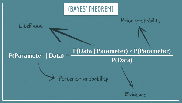
The Bayesian approach, instead, treat p as a random variable with its own distribution of possible values. The distribution can be defined by the existing evidence. The logic goes as follows. What is the probability of a given value of p, given the data? We find it, with the Bayes thm.


 , denoted
 ![E[X]](https://wikimedia.org/api/rest_v1/media/math/render/svg/e455a34363c03fc5df8208d8b81fa29e3cdd524e) , is a generalization of the weighted average and is intuitively the arithmetic mean of a large number of independentrealizations of
, is a generalization of the weighted average and is intuitively the arithmetic mean of a large number of independentrealizations of  is
is 
 is defined as the arithmetic mean of the terms
 of an individual outcome
  are unequal, then the expected value is defined to be the probability-weighted average of the
  products
  . The expected value of a general random variable involves integration in the sense of Lebesgue.
 .
.


 is the sample mean, the limiting form of the distribution of


